Курс Эндрю Ына Машинное Обучение в Стэнфордском университете (CS229 - Machine Learning)
С 2011 года на протяжении многих лет лучшим и самым популярным в мире начальным курсом по Машинному Обучению (Machine Learning) являлся одноименный бесплатный курс Эндрю Ына (Andrew Ng) на Курсере (Coursera). Andrew Ng занимал должность VP & Chief Scientist в Baidu; является Co-Chairman and Co-Founder of Coursera; co-founded and led Google Brain и an Adjunct Professor (ранее associate professor и Director of the AI Lab) в Stanford University. Курс дает базовое понимание основ Машинного Обучения. В апреле 2022 года данный курс существенно переработали и он теперь доступен на Coursera под именем «Machine Learning Specialization». Практические примеры и задания старого курса использовали Octave, что, по мнению многих, являлось основным недостатком курса. Эндрю Ын отвечал, что для вводного курса Octave проще и понятнее, чем R или Python. Но мир меняется и теперь новый курс основан на использовании Python, NumPy, scikit-learn и TensorFlow. Вот сравнительная таблица содержания старого и обновленного курсов:
| Machine Learning Course, 2011 | Machine Learning Specialization, 2022 | |
|---|---|---|
| Неделя 1 | Linear Regression with One Variable | Gradient Descent for Linear Regression |
| Неделя 2 | Linear Regression with Multiple Variables | Linear Regression using Scikit-Learn |
| Неделя 3 | Logistic Regression | Logistic Regression, Logistic Loss |
| Неделя 4 | Multi-Class Classification and Neural Networks | Neural Networks for Handwritten Digit Recognition, Binary |
| Неделя 5 | Implementation of backpropagation algorithm for Neural Networks and how to apply it to the task of Handwritten Digit Recognition | Neural Networks for Handwritten Digit Recognition, Multiclass |
| Неделя 6 | Советы по применению Машинного Обучения | |
| Неделя 7 | Support Vector Machines (SVMs) | Decision trees. Random Forests and Boosted trees (XGBoost). |
| Неделя 8 | K-means Clustering. Dimensionality Reduction. Principal Component Analysis. | Unsupervised learning: clustering and anomaly detection. K-means Clustering for image compression. |
| Неделя 9 | Anomaly Detection. Recommender Systems | Recommender systems. |
| Неделя 10 | Large-Scale Machine Learning. Example of an application of machine learning | Reinforcement Learning |
Хотя старый курс был основан на Octave, я все же для себя пришел к выводу, что повторить задания на Python просто необходимо, чтобы действительно понять и структуру представленных данных и методы решения. Мои (и не только мои) решения с использованием Python можно найти в моем репозитории на GitHub.
Данная страница создана в помощь рускоязычному сообществу и, возможно, будет полезна при прохождении данного курса, особенно для тех, кто не очень свободно владеет английским языком. Все записи сделаны на основе старого курса.
C заданиями нового курса можно ознакомится здесь.
Определение термина Машинное Обучение от Артура Самуэля: "Machine Learning is the field of study that gives computers the ability to learn without being explicitly programmed", т.е. "область исследования, которая дает компьютерам возможность учиться без явного программирования".
Определение термина Машинное Обучение от Тома Митчелла: "A computer program is said to learn from experience E with respect to some class of tasks T and performance measure P, if its performance at tasks in T, as measured by P, improves with experience E.", т.е. "говорят, что компьютерная программа учится на опыте E по отношению к некоторому классу задач T и измерению производительности P, если ее производительность при выполнении задач в T, измеренная P, улучшается с опытом E".
Пример: игра в шашки. E = опыт, полученный от многочисленных партий. T = задача игры в шашки. P = вероятность того, что программа выиграет следующую игру.
- GNU Octave (официальный сайт).
- Введение в Octave для инженеров и математиков. Авторы: Е.Р. Алексеев, О.В. Чеснокова
- Supervised learning. CS229 Lecture notes by Andrew Ng.
- Неделя 1. Градиентный спуск для линейной регрессии с одной переменной.
- Задание для первой и второй недели
- Датасет ex1data1.txt
- Подробное решение c графиками на Python с помощью Pandas и Numpy
- Решение той же задачи с помощью Scikit-Learn
- Неделя 2. Градиентный спуск для множественной линейной регрессии.
- Датасет ex1data2.txt
- Нормализация данных и решение с помощью Numpy
- Решение тех же задач первой и второй недели с помощью метода нормальных уровнений
-
Неделя 3. Функция потерь (cost funtction) и градиентный спуск для логистической
регрессии.
Неделя 3. Регуляризация. - Задание для третьей недели
- Датасет ex2data1.txt
- Логистическая регрессия по двум независимым переменным с помощью метода Градиентный спуск
- То же решение с помощью Scikit-Learn
- Датасет результатов двух тестов по контролю качества (два числовых признака) микрочипов
- Использование полиномиальных признаков в логистической регресии для построения нелинейных разделяющих поверхностей
- Пояснения к решению задачи на mlcourse.ai
- Неделя 4. Нейронные сети. Основы.
- Задание для четвертой недели. Мультиклассовая классификация.
- Датасет с 5,000 примерами рукописных цифр из базы данных MNIST
- Решение для One-vs-all Classification & Prediction
- Параметры для нейронной сети
- Неделя 5. Нейронные сети. Cost Function и Метод обратного распространения ошибки (backpropagation).
- Неделя 6. Советы по применению Машинного Обучения.
- Неделя 7. Метод Опорных Векторов или SVM (от англ. Support Vector Machines).
- Неделя 8. Кластерный анализ. Метод k-средних.
- Неделя 9. Система поиска аномалий (Anomaly Detection).
Целью моделей "Обучение с учителем" (Supervised learning) является поиск параметров (весов), которые минимизируют функцию потерь (Cost function). По размерности независимой переменной $x$ можно выделить однофакторные (univariable) и многофакторые (multivariable) модели. Если независимая переменная $x^{(i)}$ является скалярным значением, то имеем одинарную (univariate) модель. Когда независимая переменная является многомерной, то есть представлена вектором, получаем множественную (multivariate ) модель. В последующих примерах, это поиск $\theta_n$ для каждой независимой переменной $x_n$ с использованием линейной регрессии:
- Отличная статья с примерами кода на Python: Линейные модели: простая регрессия
- Начало этой статьи с описанием многообразия линейных моделей здесь
- Также советую прочитать статью Базовые принципы машинного обучения на примере линейной регрессии
- Линейные модели классификации и регрессии
Определение термина Cost function. Дать определение этого термина и показать его отличия от Loss function на русском языке, оказалось достаточно сложной задачей. Поэтому привожу определения на английском:
Loss function is usually a function defined on a data point, prediction and label, and measures the penalty. For example:- square loss $l(f(x_i|\theta),y_i) = \left (f(x_i|\theta)-y_i \right )^2$, used in linear regression
- hinge loss $l(f(x_i|\theta), y_i) = \max(0, 1-f(x_i|\theta)y_i)$, used in SVM
- 0/1 loss $l(f(x_i|\theta), y_i) = 1 \iff f(x_i|\theta) \neq y_i$, used in theoretical analysis and definition of accuracy
- Mean Squared Error $MSE(\theta) = \frac{1}{N} \sum_{i=1}^N \left (f(x_i|\theta)-y_i \right )^2$
- SVM cost function $SVM(\theta) = \|\theta\|^2 + C \sum_{i=1}^N \xi_i$ (there are additional constraints connecting $\xi_i$ with $C$ and with training set)
- MLE is a type of objective function (which you maximize)
- Divergence between classes can be an objective function but it is barely a cost function, unless you define something artificial, like 1-Divergence, and name it a cost
A loss function is a part of a cost function which is a type of an objective function.
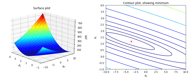
$$J(\theta) =\frac{1}{2m}\sum\limits_{i=1}^{m} \left(h_\theta(x^{(i)})-y^{(i)}\right)^2$$ где $J(\theta) =$ $J(\theta_0, \theta_1,\theta_2, ..., \theta_n)$;$h_\theta(x)=$ $\theta_0+\theta_1 x_1+\theta_2 x_2+...+\theta_n x_n$.
Если сделать так, что $x_0=1$, то $h_\theta(x)$ можно записать как $\sum\limits_{i=1}^{n} \theta_i x_i$ $=\theta^Tx$. Соответственно лучший код на Octave для этого задания:
computeCostMulti.m :
function J = computeCostMulti(X, y, theta)

  %   COMPUTECOSTMULTI Compute cost for linear regression with multiple variables
  %   J = COMPUTECOSTMULTI(X, y, theta) computes the cost of using theta as the
  %   parameter for linear regression to fit the data points in X and y

  %   Initialize some useful values
  m = length(y); % number of training examples

  %   You need to return the following variables correctly
  J = 0;

  % ====================== YOUR CODE HERE ======================
  %   Instructions: Compute the cost of a particular choice of theta
  %               You should set J to the cost.

  J = (1/(2*m))*(sum(((X*theta)-y).^2));

  % =========================================================================

end
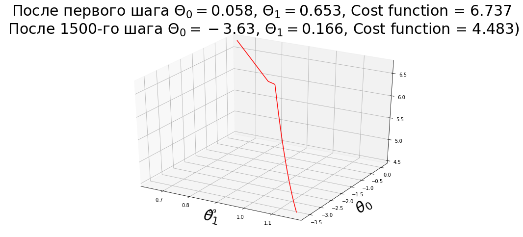
В первом задании первоначальные значения $\theta_0$ и $\theta_1$ равны нулю. Расчет функции потерь (cost function) методом наименьших квадратов на Python с моими комментариями представлен здесь. Про назначение коэффициента $\frac{1}{2m}$ в функции потерь можно прочитать в ответах на следующие вопросы:
- Почему в функции потерь (cost function) используется формула средней квадратичной ошибки (mean squared error, MSE)?
- Зачем нужно делить на $2m$?
- Функция потерь (cost function) в Методе наименьших квадратов (МНК, Ordinary Least Squares, OLS) регрессионного анализа
Градиентный спуск
- Определение градиента
- Почему вектор градиента всегда должен быть направлен в возрастающем направлении? Доказательство.
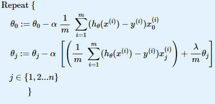
Определение термина Gradient descent (Градиентный спуск) - метод нахождения локального экстремума
(минимума или максимума) функции с помощью движения вдоль градиента. $$\theta_j := \theta_j - \alpha \frac{\partial}{\partial \theta_j} J(\theta)$$
где $j=0, 1, 2...n$, а $n$ - количество шагов, необходимых для вычисления оптимального значения $\theta$;
$\alpha$ - шаг
метода Градиентный спуск, скорость обучения. Основное правило: при каждом шаге значение $\theta_j$ должно
уменьшаться, поэтому значение $\alpha$ не должно быть слишком большим. Но если значение $\alpha$ очень
маленькое, то метод будет
работать очень долго. Поэтому всегда требуется искать золотую середину.
$\frac{\partial}{\partial \theta_j}
J(\theta)$ - частная производная,
которая равна $\frac{\partial}{\partial \theta_j} \frac{1}{2m}\sum
\limits_{i=1}^{m} \left(h_\theta(x^{(i)})-y^{(i)}\right)^2$ = $2 \cdot \frac{1}{2m}
\left(h_\theta(x^{(i)})-y^{(i)}\right)
\cdot \frac{\partial}{\partial \theta_j} \left(h_\theta(x^{(i)})-y^{(i)}\right)$ = $\frac{1}{m}
\left(h_\theta(x^{(i)})-y^{(i)}\right) \cdot \frac{\partial}{\partial \theta_j} \left(\sum \limits_{i=1}^{m}
\theta_i x^{(i)}_j -
y^{(i)}\right)$ = $\frac{1}{m} \left(h_\theta(x^{(i)})-y^{(i)}\right) x^{(i)}_j$, в итоге получаем: $$\theta_j
:= \theta_j + \alpha \frac{1}{m} \left(y^{(i)}-h_\theta(x^{(i)})\right) x^{(i)}_j$$
Код на Octave для заданий второй недели по определению шага градиентного спуска: theta = theta -((1/m) * ((X * theta) - y)' * X)' * alpha.
gradientDescentMulti.m :
function [theta, J_history] = gradientDescentMulti(X, y, theta, alpha, num_iters)

  %   GRADIENTDESCENTMULTI Performs gradient descent to learn theta
  %   theta = GRADIENTDESCENTMULTI(x, y, theta, alpha, num_iters) updates theta by
  %   taking num_iters gradient steps with learning rate alpha

  % Initialize some useful values
  m = length(y); % number of training examples
  J_history = zeros(num_iters, 1);

  for iter = 1:num_iters

  % ====================== YOUR CODE HERE ======================
  % Instructions: Perform a single gradient step on the parameter vector
  %               theta.
  %
  % Hint: While debugging, it can be useful to print out the values
  %       of the cost function (computeCostMulti) and gradient here.
  %

  %%%%%%%% CORRECT %%%%%%%%%%
  error = (X * theta) - y;
  theta = theta - ((alpha/m) * X'*error);
  %%%%%%%%%%%%%%%%%%%%%%%%%%%

  % ============================================================

  % Save the cost J in every iteration
  J_history(iter) = computeCostMulti(X, y, theta);

  end
end
Нормализация данных
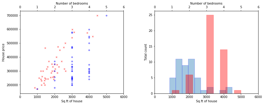
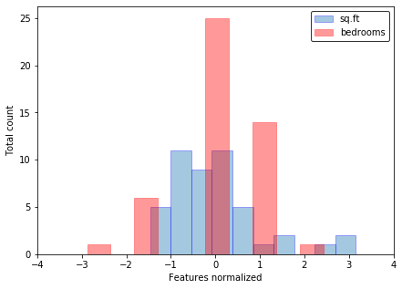
Если features (признаки) отличаются на порядки, то их масштабирование существенно ускоряет работу метода градиентного спуска. Эта процедура называется Feature scaling. Вот пример данных до и после нормализации из задачки второй недели:
featureNormalize.m :
function [X_norm, mu, sigma] = featureNormalize(X)

  %   FEATURENORMALIZE Normalizes the features in X
  %   FEATURENORMALIZE(X) returns a normalized version of X where
  %   the mean value of each feature is 0 and the standard deviation
  %   is 1. This is often a good preprocessing step to do when
  %   working with learning algorithms.

  %   You need to set these values correctly
  X_norm = X;
  mu = zeros(1, size(X, 2));
  sigma = zeros(1, size(X, 2));

  % ====================== YOUR CODE HERE ======================
  % Instructions: First, for each feature dimension, compute the mean
  %               of the feature and subtract it from the dataset,
  %               storing the mean value in mu. Next, compute the
  %               standard deviation of each feature and divide
  %               each feature by it's standard deviation, storing
  %               the standard deviation in sigma.
  %
  %               Note that X is a matrix where each column is a
  %               feature and each row is an example. You need
  %               to perform the normalization separately for
  %               each feature.
  %
  % Hint: You might find the 'mean' and 'std' functions useful.
  %

  mu = mean(X);
  sigma = std(X);
  X_norm = (X - mu)./sigma;

  % ============================================================
end
Метод нормальных уравнений. Normal Equation. $$\theta=(X^{T}X)^{-1}X^{T}y$$
На самом деле обе приведенные выше задачи целесообразнее и проще решать методом номальных уровнений. Вот эти решения. Сравнение методов нормальных уровнений и градиентного спуска для линейной регресси приведено в следующей таблице:
| Градиентный спуск | Метод нормальных уровнений |
|---|---|
| Нужно определить размер шага Градиентного спуска, т.е. коэффициент alpha | Не требуется |
| Нужно определить количество циклов (шагов, итераций) | Не требуется |
| Временная сложность алгоритма $O(kn^2)$ | Временная сложность алгоритма $O(n^3)$, нужно рассчитать обратную матрицу $X^TX$ |
| Хорошо работает, если n - большая величина | Работает медленно, если n - большая величина |
На практике, переход от использования метода нормальных уровнений (Normal Equation) к итерационному процессу (методу Градиентного Спуска), осуществляется когда n превышает 10 000.
- Вывод формулы метода нормального уравнения для линейной регрессии
- Метод нормальных уравнений и матричное исчисление. Eli Bendersky.
- Матричное исчисление на Wiki.
- Linear least squares на Wiki.
- Объяснение Метода нормальных уравнений от Алексея Григорьева.
- Что такое производная от среднеквадратичной ошибки? Sebastian Raschka.
- Подгонка модели с помощью closed-form equations vs. Gradient Descent vs Stochastic Gradient Descent vs Mini-Batch Learning. В чем же разница? Sebastian Raschka.
- Нужен ли градиентный спуск для нахождения коэффициентов линейной регрессионной модели?
- Зачем использовать градиентный спуск для линейной регрессии, когда доступно математическое решение замкнутой формы (closed-form math solution)?
- Метод нормальных уравнений и метод Ньютона.
normalEqn.m :
function [theta] = normalEqn(X, y)

  %   NORMALEQN Computes the closed-form solution to linear regression
  %   NORMALEQN(X,y) computes the closed-form solution to linear
  %   regression using the normal equations.

  theta = zeros(size(X, 2), 1);

  % ====================== YOUR CODE HERE ======================
  % Instructions: Complete the code to compute the closed form solution
  %               to linear regression and put the result in theta.
  %

  % ---------------------- Sample Solution ----------------------

  theta = pinv(X'*X)*X'*y;

  % -------------------------------------------------------------
  % ============================================================
end
Логистическая регрессия
Цель логистической регрессии, как и любого классификатора, состоит в том, чтобы выяснить, каким образом разделить данные, чтобы обеспечить точное предсказание класса данного наблюдения с использованием информации, присутствующей в его признаках (features).
Логистическая функция (сигмоида): $$\Large{h_\theta }\left( x \right) = \frac{1}{1 + {e^{ - {\theta ^T}x}}}$$
ее вероятностная интерпритация ${h _\theta }\left( {x _i} \right) = {\rm{P}}\left( {{y _i} = 1|{x _i};\theta } \right)$.
sigmoid.m :
function g = sigmoid(z)
  %SIGMOID Compute sigmoid function
  %   g = SIGMOID(z) computes the sigmoid of z.

  % You need to return the following variables correctly
  g = zeros(size(z));

  % ====================== YOUR CODE HERE ======================
  % Instructions: Compute the sigmoid of each value of z (z can be a matrix,
  %               vector or scalar).
  g = 1./(1+exp(-z));

  % =============================================================
end
predict.m :
function p = predict(theta, X)
  %PREDICT Predict whether the label is 0 or 1 using learned logistic
  %regression parameters theta
  %   p = PREDICT(theta, X) computes the predictions for X using a
  %   threshold at 0.5 (i.e., if sigmoid(theta'*x) >= 0.5, predict 1)

  m = size(X, 1); % Number of training examples

  % You need to return the following variables correctly

  p = zeros(m, 1);

  % ====================== YOUR CODE HERE ======================
  % Instructions: Complete the following code to make predictions using
  %               your learned logistic regression parameters.
  %               You should set p to a vector of 0's and 1's
  %
  % Dimentions:
  % X     =  m x (n+1)
  % theta = (n+1) x 1

  p=(sigmoid(X*theta)>=0.5);

  %p = double(sigmoid(X * theta)>=0.5);
  % =========================================================================
end
Функция потерь логистической регрессии (Cost function for logistic regression): $$J\left( \theta \right) = \frac{1}{m}\sum\limits_{i = 1}^m {\rm{Cost}({h _\theta }\left( {x _i} \right),{y _i})}$$, где $\operatorname{Cost}(h_\theta(x),y) =$ $\begin{cases} -\log(h_\theta(x)), & \text{if $y$ = 1} \\ -\log(1-h_\theta(x)), & \text{if $y$ = 0} \end{cases}$
или более кратко ${\rm{Cost}}({h _\theta }\left( x \right),y) =$ $- y\log \left( {{h _\theta }\left( x \right)} \right) -$ $\left( {1 - y} \right)\log \left( {1 - {h _\theta }\left( x \right)} \right)$.
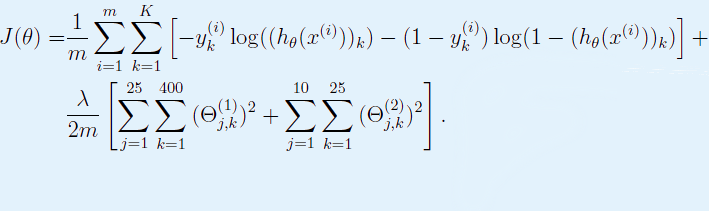
В итоге функция потерь логистической регрессии имеет вид:
Здесь подробное объяснение, как взять частную производную фунции потерь логистической регрессии в алгоритме градиентного спуска: ${\theta _j}: = {\theta _j} - \alpha \frac{\partial }{\partial {\theta _j}}J\left( \theta \right)$.
costFunction.m :
function [J, grad] = costFunction(theta, X, y)

  %   COSTFUNCTION Compute cost and gradient for logistic regression
  %   J = COSTFUNCTION(theta, X, y) computes the cost of using theta as the
  %   parameter for logistic regression and the gradient of the cost
  %   w.r.t. to the parameters.

  % Initialize some useful values
  m = length(y); % number of training examples

  % You need to return the following variables correctly
  J = 0;
  grad = zeros(size(theta));

  % ====================== YOUR CODE HERE ======================
  % Instructions: Compute the cost of a particular choice of theta.
  %               You should set J to the cost.
  %               Compute the partial derivatives and set grad to the partial
  %               derivatives of the cost w.r.t. each parameter in theta
  %
  % Note: grad should have the same dimensions as theta
  %
  %DIMENSIONS:
  %   theta = (n+1) x 1
  %   X     = m x (n+1)
  %   y     = m x 1
  %   grad  = (n+1) x 1
  %   J     = Scalar

  z = X * theta;      % m x 1
  h_x = sigmoid(z);   % m x 1

  J = (1/m)*sum((-y.*log(h_x))-((1-y).*log(1-h_x))); % scalar

  grad = (1/m)* (X'*(h_x-y));     % (n+1) x 1

  % =============================================================

end
- Градиентный спуск — метод оптимизации первого порядка (первая производная). Вот более сложные и быстрые способы оптимизации $\theta$, которые могут быть использованы вместо метода градиентного спуска:
- Conjugate gradient method (метод сопряженных градиентов). Подробное описание алгоритма в статье Jonathan Richard Shewchuk от 1994 года "Введение в метод сопряженного градиента без мучительной боли"
- Метод BFGS - Алгоритм Бройдена — Флетчера — Гольдфарба — Шанно (англ. Broyden — Fletcher — Goldfarb — Shanno algorithm)
- Метод Limited-memory BFGS - (L-BFGS or LM-BFGS)
- Обзор алгоритмов оптимизации градиентного спуска от Себастьяна Рудера - (An overview of gradient descent optimization algorithms by Sebastian Ruder)
- Поиск минимума нелинейной функции нескольких переменных без ограничения на переменные можно осуществлять с помощью встроенной в Matlab/Octave функции fminunc. Она позволяет использовать предварительно заданные командой optimset порог сходимости для значения целевой функции, вектор градиентов options, grad-obj, матрицу Гесса, функцию умножения матрицы Гесса или график разреженности матрицы Гесса целевой функции:
- Документация на MathWorks
- Практикум по решению задач оптимизации в пакете MATLAB
Регуляризация
Регуляризация в машинном обучении — метод добавления некоторой дополнительной информации к условию с целью решить некорректно поставленную задачу или предотвратить переобучение.


costFunctionReg.m :
function [J, grad] = costFunctionReg(theta, X, y, lambda)
    %COSTFUNCTIONREG Compute cost and gradient for logistic regression with regularization
  %   J = COSTFUNCTIONREG(theta, X, y, lambda) computes the cost of using
  %   theta as the parameter for regularized logistic regression and the
  %   gradient of the cost w.r.t. to the parameters.

  % Initialize some useful values
  m = length(y); % number of training examples

  % You need to return the following variables correctly
  J = 0;
  grad = zeros(size(theta));

  % ====================== YOUR CODE HERE ======================
  % Instructions: Compute the cost of a particular choice of theta.
  %               You should set J to the cost.
  %               Compute the partial derivatives and set grad to the partial
  %               derivatives of the cost w.r.t. each parameter in theta

  %DIMENSIONS:
  %   theta = (n+1) x 1
  %   X     = m x (n+1)
  %   y     = m x 1
  %   grad  = (n+1) x 1
  %   J     = Scalar

  z = X * theta;      % m x 1
  h_x = sigmoid(z);  % m x 1

  reg_term = (lambda/(2*m)) * sum(theta(2:end).^2);

  J = (1/m)*sum((-y.*log(h_x))-((1-y).*log(1-h_x))) + reg_term; % scalar

  grad(1) = (1/m)* (X(:,1)'*(h_x-y));                                  % 1 x 1
  grad(2:end) = (1/m)* (X(:,2:end)'*(h_x-y))+(lambda/m)*theta(2:end);  % n x 1

  % =============================================================
end
Неделя 4. Нейронные сети. Основы.
Логические элементы:
| INPUT | OUTPUT | ||||||
|---|---|---|---|---|---|---|---|
| A | B | AND | NAND | OR | NOR | XOR | XNOR |
| 0 | 0 | 0 | 1 | 0 | 1 | 0 | 1 |
| 0 | 1 | 0 | 1 | 1 | 0 | 1 | 0 |
| 1 | 0 | 0 | 1 | 1 | 0 | 1 | 0 |
| 1 | 1 | 1 | 0 | 1 | 0 | 0 | 1 |
Код для lrCostFunction.m такой же как и в costFunctionReg.m из предыдущего урока.
Попробуйте запустить следующие примеры кода в Octave перед решением задач этой недели:% ====================== 1 ====================== a = 1:10 b = 3 a == b % ====================== 2 ====================== Q = zeros(5,3) v = [1 2 3]' Q(2,:) = v % ====================== 3 ====================== Q = magic(3) m = size(Q,1) Q = [ones(m,1) Q]
oneVsAll.m :
function [all_theta] = oneVsAll(X, y, num_labels, lambda)
    %ONEVSALL trains multiple logistic regression classifiers and returns all
    %the classifiers in a matrix all_theta, where the i-th row of all_theta
    %corresponds to the classifier for label i
    %   [all_theta] = ONEVSALL(X, y, num_labels, lambda) trains num_labels
    %   logistic regression classifiers and returns each of these classifiers
    %   in a matrix all_theta, where the i-th row of all_theta corresponds
    %   to the classifier for label i

    % num_labels = No. of output classifier (Here, it is 10)

    % Some useful variables
    m = size(X, 1);        % No. of Training Samples == No. of Images : (Here, 5000)
    n = size(X, 2);        % No. of features == No. of pixels in each Image : (Here, 400)

    % You need to return the following variables correctly
    all_theta = zeros(num_labels, n + 1);
    %DIMENSIONS: num_labels x (input_layer_size+1) == num_labels x (no_of_features+1) == 10 x 401

    %DIMENSIONS: X = m x input_layer_size
    %Here, 1 row in X represents 1 training Image of pixel 20x20

    % Add ones to the X data matrix
    X = [ones(m, 1) X];   %DIMENSIONS: X = m x (input_layer_size+1) = m x (no_of_features+1)

    % ====================== YOUR CODE HERE ======================
    % Instructions: You should complete the following code to train num_labels
    %               logistic regression classifiers with regularization
    %               parameter lambda.
    %
    % Hint: theta(:) will return a column vector.
    %
    % Hint: You can use y == c to obtain a vector of 1's and 0's that tell you
    %       whether the ground truth is true/false for this class.
    %
    % Note: For this assignment, we recommend using fmincg to optimize the cost
    %       function. It is okay to use a for-loop (for c = 1:num_labels) to
    %       loop over the different classes.
    %
    %       fmincg works similarly to fminunc, but is more efficient when we
    %       are dealing with large number of parameters.
    %
    % Example Code for fmincg:
    %
    %     % Set Initial theta
    %     initial_theta = zeros(n + 1, 1);
    %
    %     % Set options for fminunc
    %     options = optimset('GradObj', 'on', 'MaxIter', 50);
    %
    %     % Run fmincg to obtain the optimal theta
    %     % This function will return theta and the cost
    %     [theta] = ...
    %         fmincg (@(t)(lrCostFunction(t, X, (y == c), lambda)), ...
    %                 initial_theta, options);
    %

    initial_theta = zeros(n+1, 1);
    options = optimset('GradObj', 'on', 'MaxIter', 50);

    for c=1:num_labels
    all_theta(c,:) = ...
             fmincg (@(t)(lrCostFunction(t, X, (y == c), lambda)), ...
                     initial_theta, options);
    end

    % =========================================================================
  end
predictOneVsAll.m :
  function p = predictOneVsAll(all_theta, X)
    %PREDICT Predict the label for a trained one-vs-all classifier. The labels
    %are in the range 1..K, where K = size(all_theta, 1).
    %  p = PREDICTONEVSALL(all_theta, X) will return a vector of predictions
    %  for each example in the matrix X. Note that X contains the examples in
    %  rows. all_theta is a matrix where the i-th row is a trained logistic
    %  regression theta vector for the i-th class. You should set p to a vector
    %  of values from 1..K (e.g., p = [1; 3; 1; 2] predicts classes 1, 3, 1, 2
    %  for 4 examples)

    m = size(X, 1);     % No. of Input Examples to Predict (Each row = 1 Example)
    num_labels = size(all_theta, 1); %No. of Ouput Classifier

    % You need to return the following variables correctly
    p = zeros(size(X, 1), 1);    % No_of_Input_Examples x 1 == m x 1

    % Add ones to the X data matrix
    X = [ones(m, 1) X];

    % ====================== YOUR CODE HERE ======================
    % Instructions: Complete the following code to make predictions using
    %               your learned logistic regression parameters (one-vs-all).
    %               You should set p to a vector of predictions (from 1 to
    %               num_labels).
    %
    % Hint: This code can be done all vectorized using the max function.
    %       In particular, the max function can also return the index of the
    %       max element, for more information see 'help max'. If your examples
    %       are in rows, then, you can use max(A, [], 2) to obtain the max
    %       for each row.
    %
    % num_labels = No. of output classifier (Here, it is 10)
    % DIMENSIONS:
    % all_theta = 10 x 401 = num_labels x (input_layer_size+1) == num_labels x (no_of_features+1)

    prob_mat = X * all_theta';     % 5000 x 10 == no_of_input_image x num_labels
    [prob, p] = max(prob_mat,[],2); % m  x 1
    %returns maximum element in each row  == max. probability and its index for each input image
    %p: predicted output (index)
    %prob: probability of predicted output

    %%%%%%%% WORKING: Computation per input image %%%%%%%%%
    % for i = 1:m                               % To iterate through each input sample
    %     one_image = X(i,:);                   % 1 x 401 == 1 x no_of_features
    %     prob_mat = one_image * all_theta';    % 1 x 10  == 1 x num_labels
    %     [prob, out] = max(prob_mat);
    %     %out: predicted output
    %     %prob: probability of predicted output
    %     p(i) = out;
    % end
    %%%%%%%%%%%%%%%%%%%%%%%%%%%%%%%%%%%%%%%%%%%%%%%%%%%%%%%

    %%%%%%%% WORKING %%%%%%%%%
    % for i = 1:m
    %     RX = repmat(X(i,:),num_labels,1);
    %     RX = RX .* all_theta;
    %     SX = sum(RX,2);
    %     [val, index] = max(SX);
    %     p(i) = index;
    % end
    %%%%%%%%%%%%%%%%%%%%%%%%%%
    % =========================================================================
  end
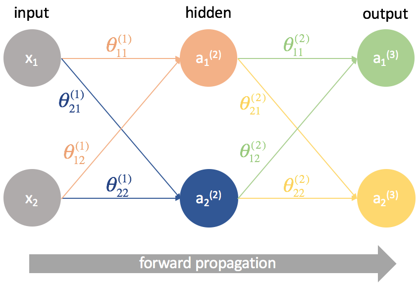
Сети прямого распространения (Feedforward neural network) (feedforward сети) - искусственные нейронные сети, в которых сигнал распространяется строго от входного слоя к выходному. В обратном направлении сигнал не распространяется.
predict.m :
  function p = predict(Theta1, Theta2, X)
    %PREDICT Predict the label of an input given a trained neural network
    %   p = PREDICT(Theta1, Theta2, X) outputs the predicted label of X given the
    %   trained weights of a neural network (Theta1, Theta2)

    % Useful values
    m = size(X, 1);
    num_labels = size(Theta2, 1);

    % You need to return the following variables correctly
    p = zeros(size(X, 1), 1);  % m x 1

    % ====================== YOUR CODE HERE ======================
    % Instructions: Complete the following code to make predictions using
    %               your learned neural network. You should set p to a
    %               vector containing labels between 1 to num_labels.
    %
    % Hint: The max function might come in useful. In particular, the max
    %       function can also return the index of the max element, for more
    %       information see 'help max'. If your examples are in rows, then, you
    %       can use max(A, [], 2) to obtain the max for each row.
    %
    %DIMENSIONS:
    % theta1 = 25 x 401
    % theta2 = 10 x 26

    % layer1 (input)  = 400 nodes + 1bias
    % layer2 (hidden) = 25 nodes + 1bias
    % layer3 (output) = 10 nodes
    %
    % theta dimensions = S_(j+1) x ((S_j)+1)
    % theta1 = 26 x 401
    % theta2 = 10 x 26

    % theta1:
    %     1st row indicates: theta corresponding to all nodes from layer1 connecting to for 1st node of layer2
    %     2nd row indicates: theta corresponding to all nodes from layer1 connecting to for 2nd node of layer2
    %     and
    %     1st Column indicates: theta corresponding to node1 from layer1 to all nodes in layer2
    %     2nd Column indicates: theta corresponding to node2 from layer1 to all nodes in layer2
    %
    % theta2:
    %     1st row indicates: theta corresponding to all nodes from layer2 connecting to for 1st node of layer3
    %     2nd row indicates: theta corresponding to all nodes from layer2 connecting to for 2nd node of layer3
    %     and
    %     1st Column indicates: theta corresponding to node1 from layer2 to all nodes in layer3
    %     2nd Column indicates: theta corresponding to node2 from layer2 to all nodes in layer3

    a1 = [ones(m,1) X]; % 5000 x 401 == no_of_input_images x no_of_features % Adding 1 in X
    %No. of rows = no. of input images
    %No. of Column = No. of features in each image

    z2 = a1 * Theta1';  % 5000 x 25
    a2 = sigmoid(z2);   % 5000 x 25

    a2 =  [ones(size(a2,1),1) a2];  % 5000 x 26

    z3 = a2 * Theta2';  % 5000 x 10
    a3 = sigmoid(z3);  % 5000 x 10

    [prob, p] = max(a3,[],2);
    %returns maximum element in each row  == max. probability and its index for each input image
    %p: predicted output (index)
    %prob: probability of predicted output

    % =========================================================================
  end
Неделя 5. Нейронные сети. Cost Function и Метод обратного распространения ошибки (англ. backpropagation).
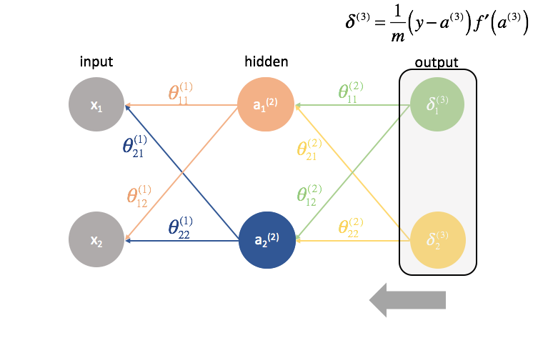
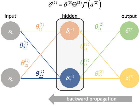
Функция потерь для нейронной сети:

Функция потерь для данной задачи, где нейронная сеть состоит из одного внутреннего слоя:
% ====================== 1 ======================
  num_labels = 5
  I = eye(num_labels)
  y = [2 3 3 1 5 4 4 4]
  Y = I(y, :)
% ====================== 2 ======================
  g= sigmoid(z).*(1-sigmoid(z));
% ====================== 3 ======================
  g = (1./(1+exp(-z))).*(1-1./(1+exp(-z)));
nnCostFunction.m :
    function [J, grad] = nnCostFunction(nn_params, ...
          input_layer_size, ...
          hidden_layer_size, ...
          num_labels, ...
          X, y, lambda)
      %NNCOSTFUNCTION Implements the neural network cost function for a two layer
      %neural network which performs classification
      %   [J grad] = NNCOSTFUNCTON(nn_params, hidden_layer_size, num_labels, ...
      %   X, y, lambda) computes the cost and gradient of the neural network. The
      %   parameters for the neural network are "unrolled" into the vector
      %   nn_params and need to be converted back into the weight matrices.
      %
      %   The returned parameter grad should be a "unrolled" vector of the
      %   partial derivatives of the neural network.
      %

      % Reshape nn_params back into the parameters Theta1 and Theta2, the weight matrices
      % for our 2 layer neural network
      % DIMENSIONS:
      % Theta1 = 25 x 401
      % Theta2 = 10 x 26

      Theta1 = reshape(nn_params(1:hidden_layer_size * (input_layer_size + 1)), ...
          hidden_layer_size, (input_layer_size + 1));

      Theta2 = reshape(nn_params((1 + (hidden_layer_size * (input_layer_size + 1))):end), ...
          num_labels, (hidden_layer_size + 1));

      % Setup some useful variables
      m = size(X, 1);

      % You need to return the following variables correctly
      J = 0;
      Theta1_grad = zeros(size(Theta1)); %25 x401
      Theta2_grad = zeros(size(Theta2)); %10 x 26

      % ====================== YOUR CODE HERE ======================
      % Instructions: You should complete the code by working through the
      %               following parts.
      %
      % Part 1: Feedforward the neural network and return the cost in the
      %         variable J. After implementing Part 1, you can verify that your
      %         cost function computation is correct by verifying the cost
      %         computed in ex4.m
      %
      % Part 2: Implement the backpropagation algorithm to compute the gradients
      %         Theta1_grad and Theta2_grad. You should return the partial derivatives of
      %         the cost function with respect to Theta1 and Theta2 in Theta1_grad and
      %         Theta2_grad, respectively. After implementing Part 2, you can check
      %         that your implementation is correct by running checkNNGradients
      %
      %         Note: The vector y passed into the function is a vector of labels
      %               containing values from 1..K. You need to map this vector into a
      %               binary vector of 1's and 0's to be used with the neural network
      %               cost function.
      %
      %         Hint: We recommend implementing backpropagation using a for-loop
      %               over the training examples if you are implementing it for the
      %               first time.
      %
      % Part 3: Implement regularization with the cost function and gradients.
      %
      %         Hint: You can implement this around the code for
      %               backpropagation. That is, you can compute the gradients for
      %               the regularization separately and then add them to Theta1_grad
      %               and Theta2_grad from Part 2.
      %

      %%%%%%%%%%% Part 1: Calculating J w/o Regularization %%%%%%%%%%%%%%%

      X = [ones(m,1), X];  % Adding 1 as first column in X

      a1 = X; % 5000 x 401

      z2 = a1 * Theta1';  % m x hidden_layer_size == 5000 x 25
      a2 = sigmoid(z2); % m x hidden_layer_size == 5000 x 25
      a2 = [ones(size(a2,1),1), a2]; % Adding 1 as first column in z = (Adding bias unit) % m x (hidden_layer_size + 1) == 5000 x 26

      z3 = a2 * Theta2';  % m x num_labels == 5000 x 10
      a3 = sigmoid(z3); % m x num_labels == 5000 x 10

      %Converting y into vector of 0's and 1's for multi-class classification
      y = eye(num_labels)(y,:);

      %Costfunction Without regularization
      J = (1/m) * sum(sum((-y.*log(a3))-((1-y).*log(1-a3))));  %scalar


      %%%%%%%%%%% Part 2: Implementing Backpropogation for Theta_gra w/o Regularization %%%%%%%%%%%%%

      %%%%%%% WORKING: Backpropogation using for loop %%%%%%%
      % for t=1:m
      %     % Here X is including 1 column at begining
      %
      %     % for layer-1
      %     a1 = X(t,:)'; % (n+1) x 1 == 401 x 1
      %
      %     % for layer-2
      %     z2 = Theta1 * a1;  % hidden_layer_size x 1 == 25 x 1
      %     a2 = [1; sigmoid(z2)]; % (hidden_layer_size+1) x 1 == 26 x 1
      %
      %     % for layer-3
      %     z3 = Theta2 * a2; % num_labels x 1 == 10 x 1
      %     a3 = sigmoid(z3); % num_labels x 1 == 10 x 1
      %
      %     yVector = (1:num_labels)'==y(t); % num_labels x 1 == 10 x 1
      %
      %     %calculating delta values
      %     delta3 = a3 - yVector; % num_labels x 1 == 10 x 1
      %
      %     delta2 = (Theta2' * delta3) .* [1; sigmoidGradient(z2)]; % (hidden_layer_size+1) x 1 == 26 x 1
      %
      %     delta2 = delta2(2:end); % hidden_layer_size x 1 == 25 x 1 %Removing delta2 for bias node
      %
      %     % delta_1 is not calculated because we do not associate error with the input
      %
      %     % CAPITAL delta update
      %     Theta1_grad = Theta1_grad + (delta2 * a1'); % 25 x 401
      %     Theta2_grad = Theta2_grad + (delta3 * a2'); % 10 x 26
      %
      % end
      %
      % Theta1_grad = (1/m) * Theta1_grad; % 25 x 401
      % Theta2_grad = (1/m) * Theta2_grad; % 10 x 26
      %%%%%%%%%%%%%%%%%%%%%%%%%%%%%%%%%%%%%%%%%%%%

      %%%%%% WORKING: Backpropogation (Vectorized Implementation) %%%%%%%
      % Here X is including 1 column at begining
      A1 = X; % 5000 x 401

      Z2 = A1 * Theta1';  % m x hidden_layer_size == 5000 x 25
      A2 = sigmoid(Z2); % m x hidden_layer_size == 5000 x 25
      A2 = [ones(size(A2,1),1), A2]; % Adding 1 as first column in z = (Adding bias unit) % m x (hidden_layer_size + 1) == 5000 x 26

      Z3 = A2 * Theta2';  % m x num_labels == 5000 x 10
      A3 = sigmoid(Z3); % m x num_labels == 5000 x 10

      DELTA3 = A3 - y; % 5000 x 10
      DELTA2 = (DELTA3 * Theta2) .* [ones(size(Z2,1),1) sigmoidGradient(Z2)]; % 5000 x 26
      DELTA2 = DELTA2(:,2:end); % 5000 x 25 %Removing delta2 for bias node

      Theta1_grad = (1/m) * (DELTA2' * A1); % 25 x 401
      Theta2_grad = (1/m) * (DELTA3' * A2); % 10 x 26

      %%%%%%%%%%%% WORKING: DIRECT CALCULATION OF THETA GRADIENT WITH REGULARISATION %%%%%%%%%%%
      % %Regularization term is later added in Part 3
      % Theta1_grad = (1/m) * Theta1_grad + (lambda/m) * [zeros(size(Theta1, 1), 1) Theta1(:,2:end)]; % 25 x 401
      % Theta2_grad = (1/m) * Theta2_grad + (lambda/m) * [zeros(size(Theta2, 1), 1) Theta2(:,2:end)]; % 10 x 26
      %%%%%%%%%%%%%%%%%%%%%%%%%%%%%%%%%%%%%%%%%%%%%%%%%%%%%%%%%%%%%%%%%%%%%%%%%%%%%%%%%%%%%%%%%%


      %%%%%%%%%%%% Part 3: Adding Regularisation term in J and Theta_grad %%%%%%%%%%%%%
      reg_term = (lambda/(2*m)) * (sum(sum(Theta1(:,2:end).^2)) + sum(sum(Theta2(:,2:end).^2))); %scalar

      %Costfunction With regularization
      J = J + reg_term; %scalar

      %Calculating gradients for the regularization
      Theta1_grad_reg_term = (lambda/m) * [zeros(size(Theta1, 1), 1) Theta1(:,2:end)]; % 25 x 401
      Theta2_grad_reg_term = (lambda/m) * [zeros(size(Theta2, 1), 1) Theta2(:,2:end)]; % 10 x 26

      %Adding regularization term to earlier calculated Theta_grad
      Theta1_grad = Theta1_grad + Theta1_grad_reg_term;
      Theta2_grad = Theta2_grad + Theta2_grad_reg_term;

      % -------------------------------------------------------------

      % =========================================================================

      % Unroll gradients
      grad = [Theta1_grad(:) ; Theta2_grad(:)];

    end
Неделя 6. Советы по применению Машинного Обучения.
linearRegCostFunction.m :
function [J, grad] = linearRegCostFunction(X, y, theta, lambda)
  %LINEARREGCOSTFUNCTION Compute cost and gradient for regularized linear
  %regression with multiple variables
  %   [J, grad] = LINEARREGCOSTFUNCTION(X, y, theta, lambda) computes the
  %   cost of using theta as the parameter for linear regression to fit the
  %   data points in X and y. Returns the cost in J and the gradient in grad

  % Initialize some useful values
  m = length(y); % number of training examples

  % You need to return the following variables correctly
  J = 0;
  grad = zeros(size(theta));

  % ====================== YOUR CODE HERE ======================
  % Instructions: Compute the cost and gradient of regularized linear
  %               regression for a particular choice of theta.
  %
  %               You should set J to the cost and grad to the gradient.
  %DIMENSIONS:
  %   X = 12x2 = m x 1
  %   y = 12x1 = m x 1
  %   theta = 2x1 = (n+1) x 1
  %   grad = 2x1 = (n+1) x 1

  h_x = X * theta; % 12x1
  J = (1/(2*m))*sum((h_x - y).^2) + (lambda/(2*m))*sum(theta(2:end).^2); % scalar

  % grad(1) = (1/m)*sum((h_x-y).*X(:,1)); % scalar == 1x1
  grad(1) = (1/m)*(X(:,1)'*(h_x-y)); % scalar == 1x1
  grad(2:end) = (1/m)*(X(:,2:end)'*(h_x-y)) + (lambda/m)*theta(2:end); % n x 1
  % =========================================================================

  grad = grad(:);

end
learningCurve.m :
function [error_train, error_val] = ...
      learningCurve(X, y, Xval, yval, lambda)
  %LEARNINGCURVE Generates the train and cross validation set errors needed
  %to plot a learning curve
  %   [error_train, error_val] = ...
  %       LEARNINGCURVE(X, y, Xval, yval, lambda) returns the train and
  %       cross validation set errors for a learning curve. In particular,
  %       it returns two vectors of the same length - error_train and
  %       error_val. Then, error_train(i) contains the training error for
  %       i examples (and similarly for error_val(i)).
  %
  %   In this function, you will compute the train and test errors for
  %   dataset sizes from 1 up to m. In practice, when working with larger
  %   datasets, you might want to do this in larger intervals.
  %

  % Number of training examples
  m = size(X, 1);

  % You need to return these values correctly
  error_train = zeros(m, 1);
  error_val   = zeros(m, 1);

  % ====================== YOUR CODE HERE ======================
  % Instructions: Fill in this function to return training errors in
  %               error_train and the cross validation errors in error_val.
  %               i.e., error_train(i) and
  %               error_val(i) should give you the errors
  %               obtained after training on i examples.
  %
  % Note: You should evaluate the training error on the first i training
  %       examples (i.e., X(1:i, :) and y(1:i)).
  %
  %       For the cross-validation error, you should instead evaluate on
  %       the _entire_ cross validation set (Xval and yval).
  %
  % Note: If you are using your cost function (linearRegCostFunction)
  %       to compute the training and cross validation error, you should
  %       call the function with the lambda argument set to 0.
  %       Do note that you will still need to use lambda when running
  %       the training to obtain the theta parameters.
  %
  % Hint: You can loop over the examples with the following:
  %
  %       for i = 1:m
  %           % Compute train/cross validation errors using training examples
  %           % X(1:i, :) and y(1:i), storing the result in
  %           % error_train(i) and error_val(i)
  %           ....
  %
  %       end
  %

  % ---------------------- Sample Solution ----------------------

  %DIMENSIONS:
  %   error_train = m x 1
  %   error_val   = m x 1

  for i = 1:m
      Xtrain = X(1:i,:);
      ytrain = y(1:i);

      theta = trainLinearReg(Xtrain, ytrain, lambda);

      error_train(i) = linearRegCostFunction(Xtrain, ytrain, theta, 0); %for lambda = 0;
      error_val(i)   = linearRegCostFunction(Xval, yval, theta, 0); %for lambda = 0;
  end

  % -------------------------------------------------------------

  % =========================================================================

end
polyFeatures.m :
function [X_poly] = polyFeatures(X, p)
  %POLYFEATURES Maps X (1D vector) into the p-th power
  %   [X_poly] = POLYFEATURES(X, p) takes a data matrix X (size m x 1) and
  %   maps each example into its polynomial features where
  %   X_poly(i, :) = [X(i) X(i).^2 X(i).^3 ...  X(i).^p];
  %


  % You need to return the following variables correctly.
  X_poly = zeros(numel(X), p); % m x p

  % ====================== YOUR CODE HERE ======================
  % Instructions: Given a vector X, return a matrix X_poly where the p-th
  %               column of X contains the values of X to the p-th power.
  %
  %
  % Here, X does not include X0 == 1 column

  %%%% WORKING: Using for loop %%%%%%
  % for i = 1:p
  %     X_poly(:,i) = X(:,1).^i;
  % end
  %%%%%%%%%%%%%%%%%%%%%%%%%%%%%%%%%%%

  X_poly(:,1:p) = X(:,1).^(1:p); % w/o for loop

  % =========================================================================
end
validationCurve.m :
function [lambda_vec, error_train, error_val] = ...
      validationCurve(X, y, Xval, yval)
  %VALIDATIONCURVE Generate the train and validation errors needed to
  %plot a validation curve that we can use to select lambda
  %   [lambda_vec, error_train, error_val] = ...
  %       VALIDATIONCURVE(X, y, Xval, yval) returns the train
  %       and validation errors (in error_train, error_val)
  %       for different values of lambda. You are given the training set (X,
  %       y) and validation set (Xval, yval).
  %

  % Selected values of lambda (you should not change this)
  lambda_vec = [0 0.001 0.003 0.01 0.03 0.1 0.3 1 3 10]';

  % You need to return these variables correctly.
  error_train = zeros(length(lambda_vec), 1);
  error_val = zeros(length(lambda_vec), 1);

  % ====================== YOUR CODE HERE ======================
  % Instructions: Fill in this function to return training errors in
  %               error_train and the validation errors in error_val. The
  %               vector lambda_vec contains the different lambda parameters
  %               to use for each calculation of the errors, i.e,
  %               error_train(i), and error_val(i) should give
  %               you the errors obtained after training with
  %               lambda = lambda_vec(i)
  %
  % Note: You can loop over lambda_vec with the following:
  %
  %       for i = 1:length(lambda_vec)
  %           lambda = lambda_vec(i);
  %           % Compute train / val errors when training linear
  %           % regression with regularization parameter lambda
  %           % You should store the result in error_train(i)
  %           % and error_val(i)
  %           ....
  %
  %       end
  %
  %

  % Here, X & Xval are already including x0 i.e 1's column in it

  m = size(X, 1);

  %% %%%%% WORKING: BUT UNNECESSARY for loop for i is inovolved %%%%%%%%%%%
  % for i = 1:m
  %     for j = 1:length(lambda_vec);
  %         lambda = lambda_vec(j);
  %         Xtrain = X(1:i,:);
  %         ytrain = y(1:i);
  %
  %         theta = trainLinearReg(Xtrain, ytrain, lambda);
  %
  %         error_train(j) = linearRegCostFunction(Xtrain, ytrain, theta, 0); % lambda = 0;
  %         error_val(j)   = linearRegCostFunction(Xval, yval, theta, 0); % lambda = 0;
  %     end
  % end
  %%%%%%%%%%%%%%%%%%%%%%%%%%%%%%%%%%%%%%%%%%%%%%%%%%%%%%%%%%%%%%%%%%%%%%%%

  %% %%%%%%% WORKING: BUT UNNECESSARY for loop for i is inovolved %%%%%%%%%%%
  % for j = 1:length(lambda_vec)
  %     lambda = lambda_vec(j);
  %     for i = 1:m
  %         Xtrain = X(1:i,:);
  %         ytrain = y(1:i);
  %
  %         theta = trainLinearReg(Xtrain, ytrain, lambda);
  %
  %         error_train(j) = linearRegCostFunction(Xtrain, ytrain, theta, 0); % lambda = 0;
  %         error_val(j)   = linearRegCostFunction(Xval, yval, theta, 0); % lambda = 0;
  %     end
  % end
  %%%%%%%%%%%%%%%%%%%%%%%%%%%%%%%%%%%%%%%%%%%%%%%%%%%%%%%%%%%%%%%%%%%%%%%%%%

  %% %%% NOT WORKING: BUT UNNECESSARY for loop inside learningCurve function is inovolved %%%%%%
  % for j = 1:length(lambda_vec)
  %     lambda = lambda_vec(j);
  %
  %     [error_train_temp, error_val_temp] = ...
  %     learningCurve(X, y, ...
  %                   Xval, yval, ...
  %                   lambda);
  %
  %     error_train(j) = error_train_temp(end);
  %     error_val(j) = error_val_temp(end);
  % end
  %%%%%%%%%%%%%%%%%%%%%%%%%%%%%%%%%%%%%%%%%%%%%%%%%%%%%%%%%%%%%%%%%%%%%%%%%%%%%%%%%%%%%%%%%%%%%


  %% %%%%% WORKING: OPTIMISED (Only 1 for loop) %%%%%%%%%%%
  for j = 1:length(lambda_vec)
      lambda = lambda_vec(j);

      theta = trainLinearReg(X, y, lambda);
      error_train(j) = linearRegCostFunction(X, y, theta, 0); % lambda = 0;
      error_val(j)   = linearRegCostFunction(Xval, yval, theta, 0); % lambda = 0
  end
  %%%%%%%%%%%%%%%%%%%%%%%%%%%%%%%%%%%%%%%%%%%%%%%%%%%%%%%%

  % =========================================================================

end
Неделя 7. Метод Опорных Векторов или SVM (от англ. Support Vector Machines).
- История развития метода опорных векторов.
- Метод опорных векторов (Support Vector Machine — SVM). Ядерный трюк (kernel trick). Теорема Мерсера.
- Машина опорных векторов.
- Support Vector Machine (SVM) learning algorithm. CS229 Lecture notes by Andrew Ng.
- SVM tutorial by Alexey Nefedov.
- Support Vector Machines Succinctly by Alexandre Kowalczyk.
- Подробное объяснение работы метода опорных векторов от Tristan Fletcher.
- Сравнение метода опорных векторов и логистической регрессии.
gaussianKernel.m:
function sim = gaussianKernel(x1, x2, sigma)
  %RBFKERNEL returns a radial basis function kernel between x1 and x2
  %   sim = gaussianKernel(x1, x2) returns a gaussian kernel between x1 and x2
  %   and returns the value in sim

  % Ensure that x1 and x2 are column vectors
  x1 = x1(:); x2 = x2(:);

  % You need to return the following variables correctly.
  sim = 0;

  % ====================== YOUR CODE HERE ======================
  % Instructions: Fill in this function to return the similarity between x1
  %               and x2 computed using a Gaussian kernel with bandwidth
  %               sigma
  %
  %

  sim = exp(-1*sum(abs(x1-x2).^2)/(2*sigma^2));

  % =============================================================
end
dataset3Params.m:
function [C, sigma] = dataset3Params(X, y, Xval, yval)
  %DATASET3PARAMS returns your choice of C and sigma for Part 3 of the exercise
  %where you select the optimal (C, sigma) learning parameters to use for SVM
  %with RBF kernel
  %   [C, sigma] = DATASET3PARAMS(X, y, Xval, yval) returns your choice of C and
  %   sigma. You should complete this function to return the optimal C and
  %   sigma based on a cross-validation set.
  %

  % You need to return the following variables correctly.
  C = 1;
  sigma = 0.3;

  % ====================== YOUR CODE HERE ======================
  % Instructions: Fill in this function to return the optimal C and sigma
  %               learning parameters found using the cross validation set.
  %               You can use svmPredict to predict the labels on the cross
  %               validation set. For example,
  %                   predictions = svmPredict(model, Xval);
  %               will return the predictions on the cross validation set.
  %
  %  Note: You can compute the prediction error using
  %        mean(double(predictions ~= yval))
  %

  %% %%%%%%%%%% WORKING: SOLUTION1 %%%%%%%%%%
  % C_list     = [0.01 0.03 0.1 0.3 1 3 10 30]';
  % sigma_list = [0.01 0.03 0.1 0.3 1 3 10 30]';
  %
  % prediction_error = zeros(length(C_list), length(sigma_list));
  % for i = 1:length(C_list)
  %     for j = 1: length(sigma_list)
  %         C_test = C_list(i);
  %         sigma_test = sigma_list(j);
  %         model = svmTrain(X, y, C_test, @(x1, x2) gaussianKernel(x1, x2, sigma_test));
  %         predictions = svmPredict(model, Xval);
  %         prediction_error(i,j) = mean(double(predictions ~= yval));
  %     end
  % end
  %
  % % Finding row and col corresponding to min(prediction_error)
  % [values, row_index]=min(prediction_error);
  % [~ ,col] = min(values);
  % row = row_index(col);
  %
  % % C and sigma corresponding to min(prediction_error)
  % C = C_list(row);
  % sigma = sigma_list(col);
  %%%%%%%%%%%%%%%%%%%%%%%%%%%%%%%%%%%%%%%%%%


  %% %%%%%%%%%% WORKING: SOLUION 2 %%%%%%%%%%%%%%
  C_list     = [0.01 0.03 0.1 0.3 1 3 10 30]';
  sigma_list = [0.01 0.03 0.1 0.3 1 3 10 30]';

  prediction_error = zeros(length(C_list), length(sigma_list));
  result = zeros(length(C_list)+length(sigma_list),3);
  row = 1;

  for i = 1:length(C_list)
      for j = 1: length(sigma_list)
          C_test = C_list(i);
          sigma_test = sigma_list(j);

          model = svmTrain(X, y, C_test, @(x1, x2) gaussianKernel(x1, x2, sigma_test));
          predictions = svmPredict(model, Xval);
          prediction_error(i,j) = mean(double(predictions ~= yval));

          result(row,:) = [prediction_error(i,j), C_test, sigma_test];
          row = row + 1;
      end
  end

  % Sorting prediction_error in ascending order
  sorted_result = sortrows(result, 1);

  % C and sigma corresponding to min(prediction_error)
  C = sorted_result(1,2);
  sigma = sorted_result(1,3);
  %%%%%%%%%%%%%%%%%%%%%%%%%%%%%%%%%%%%%%%%%%
  % =========================================================================
end
processEmail.m:
function word_indices = processEmail(email_contents)
  %PROCESSEMAIL preprocesses a the body of an email and
  %returns a list of word_indices
  %   word_indices = PROCESSEMAIL(email_contents) preprocesses
  %   the body of an email and returns a list of indices of the
  %   words contained in the email.
  %

  % Load Vocabulary
  vocabList = getVocabList();

  % Init return value
  word_indices = [];

  % ========================== Preprocess Email ===========================

  % Find the Headers ( \n\n and remove )
  % Uncomment the following lines if you are working with raw emails with the
  % full headers

  % hdrstart = strfind(email_contents, ([char(10) char(10)]));
  % email_contents = email_contents(hdrstart(1):end);

  % Lower case
  email_contents = lower(email_contents);

  % Strip all HTML
  % Looks for any expression that starts with < and ends with > and replace
  % and does not have any < or > in the tag it with a space
  email_contents = regexprep(email_contents, '<[^<>]+>', ' ');

  % Handle Numbers
  % Look for one or more characters between 0-9
  email_contents = regexprep(email_contents, '[0-9]+', 'number');

  % Handle URLS
  % Look for strings starting with http:// or https://
  email_contents = regexprep(email_contents, ...
      '(http|https)://[^\s]*', 'httpaddr');

  % Handle Email Addresses
  % Look for strings with @ in the middle
  email_contents = regexprep(email_contents, '[^\s]+@[^\s]+', 'emailaddr');

  % Handle $ sign
  email_contents = regexprep(email_contents, '[$]+', 'dollar');


  % ========================== Tokenize Email ===========================

  % Output the email to screen as well
  fprintf('\n==== Processed Email ====\n\n');

  % Process file
  l = 0;

  while ~isempty(email_contents)

    % Tokenize and also get rid of any punctuation
    [str, email_contents] = ...
        strtok(email_contents, ...
        [' @$/#.-:&*+=[]?!(){},''">_<;%' char(10) char(13)]);

    % Remove any non alphanumeric characters
    str = regexprep(str, '[^a-zA-Z0-9]', '');

    % Stem the word
    % (the porterStemmer sometimes has issues, so we use a try catch block)
    try str = porterStemmer(strtrim(str));
    catch str = ''; continue;
    end;

    % Skip the word if it is too short
    if length(str) < 1
        continue;
    end

    % Look up the word in the dictionary and add to word_indices if
    % found
    % ====================== YOUR CODE HERE ======================
    % Instructions: Fill in this function to add the index of str to
    %               word_indices if it is in the vocabulary. At this point
    %               of the code, you have a stemmed word from the email in
    %               the variable str. You should look up str in the
    %               vocabulary list (vocabList). If a match exists, you
    %               should add the index of the word to the word_indices
    %               vector. Concretely, if str = 'action', then you should
    %               look up the vocabulary list to find where in vocabList
    %               'action' appears. For example, if vocabList{18} =
    %               'action', then, you should add 18 to the word_indices
    %               vector (e.g., word_indices = [word_indices ; 18]; ).
    %
    % Note: vocabList{idx} returns a the word with index idx in the
    %       vocabulary list.
    %
    % Note: You can use strcmp(str1, str2) to compare two strings (str1 and
    %       str2). It will return 1 only if the two strings are equivalent.
    %

    %% %%%%% WORKING: SOLUTION %%%%%%%%%%
    % find index of the word in vocabList (if Exist)
    index = find(strcmp(str,vocabList),1);

    % Add the index in the vector word_indices
    word_indices = [word_indices; index];

    %% =============================================================

    % Print to screen, ensuring that the output lines are not too long
    if (l + length(str) + 1) > 78
        fprintf('\n');
        l = 0;
    end
    fprintf('%s ', str);
    l = l + length(str) + 1;

  end

  % Print footer
  fprintf('\n\n=========================\n');

end
emailFeatures.m
function x = emailFeatures(word_indices)
  %EMAILFEATURES takes in a word_indices vector and produces a feature vector
  %from the word indices
  %   x = EMAILFEATURES(word_indices) takes in a word_indices vector and
  %   produces a feature vector from the word indices.

  % Total number of words in the dictionary
  n = 1899;

  % You need to return the following variables correctly.
  x = zeros(n, 1);

  % ====================== YOUR CODE HERE ======================
  % Instructions: Fill in this function to return a feature vector for the
  %               given email (word_indices). To help make it easier to
  %               process the emails, we have have already pre-processed each
  %               email and converted each word in the email into an index in
  %               a fixed dictionary (of 1899 words). The variable
  %               word_indices contains the list of indices of the words
  %               which occur in one email.
  %
  %               Concretely, if an email has the text:
  %
  %                  The quick brown fox jumped over the lazy dog.
  %
  %               Then, the word_indices vector for this text might look
  %               like:
  %
  %                   60  100   33   44   10     53  60  58   5
  %
  %               where, we have mapped each word onto a number, for example:
  %
  %                   the   -- 60
  %                   quick -- 100
  %                   ...
  %
  %              (note: the above numbers are just an example and are not the
  %               actual mappings).
  %
  %              Your task is take one such word_indices vector and construct
  %              a binary feature vector that indicates whether a particular
  %              word occurs in the email. That is, x(i) = 1 when word i
  %              is present in the email. Concretely, if the word 'the' (say,
  %              index 60) appears in the email, then x(60) = 1. The feature
  %              vector should look like:
  %
  %              x = [ 0 0 0 0 1 0 0 0 ... 0 0 0 0 1 ... 0 0 0 1 0 ..];
  %
  %

  %% WORKING: SOLUTION 1 %%%%%%
  % for i = 1:length(word_indices)
  %     x1 = ([1:n] == word_indices(i));
  %     x = x | x1';
  % end

  %% WORKING: SOLUTION 2 %%%%%%
  for i = 1:length(word_indices)
      x(word_indices(i)) = 1;
  end
  % =========================================================================
end
Неделя 8. Кластерный анализ. Метод k-средних.
findClosestCentroids.m :
function idx = findClosestCentroids(X, centroids)
  %FINDCLOSESTCENTROIDS computes the centroid memberships for every example
  %   idx = FINDCLOSESTCENTROIDS (X, centroids) returns the closest centroids
  %   in idx for a dataset X where each row is a single example. idx = m x 1
  %   vector of centroid assignments (i.e. each entry in range [1..K])
  %

  % Set K
  K = size(centroids, 1); % K x 1 == 3 x 1

  % You need to return the following variables correctly.
  idx = zeros(size(X,1), 1);  % m x 1 == 300 x 1

  % ====================== YOUR CODE HERE ======================
  % Instructions: Go over every example, find its closest centroid, and store
  %               the index inside idx at the appropriate location.
  %               Concretely, idx(i) should contain the index of the centroid
  %               closest to example i. Hence, it should be a value in the
  %               range 1..K
  %
  % Note: You can use a for-loop over the examples to compute this.
  %
  % DIMENSIONS:
  %    centroids = K x no. of features = 3 x 2

  for i = 1:size(X,1)
      temp = zeros(K,1);
      for j = 1:K
          temp(j)=sqrt(sum((X(i,:)-centroids(j,:)).^2));
      end
      [~,idx(i)] = min(temp);
  end

  % =============================================================
end
computeCentroids.m :
function centroids = computeCentroids(X, idx, K)
  %COMPUTECENTROIDS returns the new centroids by computing the means of the
  %data points assigned to each centroid.
  %   centroids = COMPUTECENTROIDS(X, idx, K) returns the new centroids by
  %   computing the means of the data points assigned to each centroid. It is
  %   given a dataset X where each row is a single data point, a vector
  %   idx of centroid assignments (i.e. each entry in range [1..K]) for each
  %   example, and K, the number of centroids. You should return a matrix
  %   centroids, where each row of centroids is the mean of the data points
  %   assigned to it.
  %

  % Useful variables
  [m n] = size(X);

  % You need to return the following variables correctly.
  centroids = zeros(K, n);


  % ====================== YOUR CODE HERE ======================
  % Instructions: Go over every centroid and compute mean of all points that
  %               belong to it. Concretely, the row vector centroids(i, :)
  %               should contain the mean of the data points assigned to
  %               centroid i.
  %
  % Note: You can use a for-loop over the centroids to compute this.
  %
  % DIMENSIONS:
  %    X =  m x n
  %    centroids = K x n

  %% %%%%%% WORKING: SOLUTION1 %%%%%%%%%
  % for i = 1:K
  %     idx_i = find(idx==i);       %indexes of all the input which belongs to cluster j
  %     centroids(i,:)=(1/length(idx_i))*sum(X(idx_i,:)); %calculating mean manually
  % end
  %%%%%%%%%%%%%%%%%%%%%%%%%%%%%%%%%%%%%%

  %% %%%%%% WORKING: SOLUTION 2 %%%%%%%%
  for i = 1:K
      idx_i = find(idx==i);       %indexes of all the input which belongs to cluster j
      centroids(i,:) = mean(X(idx_i,:)); % calculating mean using built-in function
  end
  %%%%%%%%%%%%%%%%%%%%%%%%%%%%%%%%%%%%%%
  % =============================================================
end
pca.m :
function [U, S] = pca(X)
  %PCA Run principal component analysis on the dataset X
  %   [U, S, X] = pca(X) computes eigenvectors of the covariance matrix of X
  %   Returns the eigenvectors U, the eigenvalues (on diagonal) in S
  %

  % Useful values
  [m, n] = size(X);

  % You need to return the following variables correctly.
  U = zeros(n);
  S = zeros(n);

  % ====================== YOUR CODE HERE ======================
  % Instructions: You should first compute the covariance matrix. Then, you
  %               should use the "svd" function to compute the eigenvectors
  %               and eigenvalues of the covariance matrix.
  %
  % Note: When computing the covariance matrix, remember to divide by m (the
  %       number of examples).
  %
  % DIMENSIONS:
  %    X = m x n

  Sigma = (1/m)*(X'*X); % n x n
  [U, S, V] = svd(Sigma);

  % =========================================================================
end
projectData.m :
function Z = projectData(X, U, K)
  %PROJECTDATA Computes the reduced data representation when projecting only
  %on to the top k eigenvectors
  %   Z = projectData(X, U, K) computes the projection of
  %   the normalized inputs X into the reduced dimensional space spanned by
  %   the first K columns of U. It returns the projected examples in Z.
  %

  % You need to return the following variables correctly.
  Z = zeros(size(X, 1), K);

  % ====================== YOUR CODE HERE ======================
  % Instructions: Compute the projection of the data using only the top K
  %               eigenvectors in U (first K columns).
  %               For the i-th example X(i,:), the projection on to the k-th
  %               eigenvector is given as follows:
  %                    x = X(i, :)';
  %                    projection_k = x' * U(:, k);
  %
  % DIMENSIONS:
  %    X = m x n
  %    U = n x n
  %    U_reduce = n x K
  %    K = scalar

  U_reduce = U(:,[1:K]);   % n x K
  Z = X * U_reduce;        % m x k

  % =============================================================
end
recoverData.m :
function X_rec = recoverData(Z, U, K)
  %RECOVERDATA Recovers an approximation of the original data when using the
  %projected data
  %   X_rec = RECOVERDATA(Z, U, K) recovers an approximation the
  %   original data that has been reduced to K dimensions. It returns the
  %   approximate reconstruction in X_rec.
  %

  % You need to return the following variables correctly.
  X_rec = zeros(size(Z, 1), size(U, 1));

  % ====================== YOUR CODE HERE ======================
  % Instructions: Compute the approximation of the data by projecting back
  %               onto the original space using the top K eigenvectors in U.
  %
  %               For the i-th example Z(i,:), the (approximate)
  %               recovered data for dimension j is given as follows:
  %                    v = Z(i, :)';
  %                    recovered_j = v' * U(j, 1:K)';
  %
  %               Notice that U(j, 1:K) is a row vector.
  %
  % DIMENSIONS:
  %    Z = m x K
  %    U = n x n
  %    U_reduce = n x k
  %    K = scalar
  %    X_rec = m x n

  U_reduce = U(:,1:K);   % n x k
  X_rec = Z * U_reduce'; % m x n

  % =============================================================
end
Неделя 9. Системы поиска аномалий (Anomaly Detection) и Рекомендательные системы .
estimateGaussian.m :
function [mu sigma2] = estimateGaussian(X)
    %ESTIMATEGAUSSIAN This function estimates the parameters of a
    %Gaussian distribution using the data in X
    %   [mu sigma2] = estimateGaussian(X),
    %   The input X is the dataset with each n-dimensional data point in one row
    %   The output is an n-dimensional vector mu, the mean of the data set
    %   and the variances sigma^2, an n x 1 vector
    %

    % Useful variables
    [m, n] = size(X);

    % You should return these values correctly
    mu = zeros(n, 1);
    sigma2 = zeros(n, 1);

    % ====================== YOUR CODE HERE ======================
    % Instructions: Compute the mean of the data and the variances
    %               In particular, mu(i) should contain the mean of
    %               the data for the i-th feature and sigma2(i)
    %               should contain variance of the i-th feature.
    %

    mu = ((1/m)*sum(X))';
    sigma2 = ((1/m)*sum((X-mu').^2))';

    % =============================================================
  end
selectThreshold.m :
function [bestEpsilon bestF1] = selectThreshold(yval, pval)
  %SELECTTHRESHOLD Find the best threshold (epsilon) to use for selecting
  %outliers
  %   [bestEpsilon bestF1] = SELECTTHRESHOLD(yval, pval) finds the best
  %   threshold to use for selecting outliers based on the results from a
  %   validation set (pval) and the ground truth (yval).
  %

  bestEpsilon = 0;
  bestF1 = 0;
  F1 = 0;

  stepsize = (max(pval) - min(pval)) / 1000;
  for epsilon = min(pval):stepsize:max(pval)

      % ====================== YOUR CODE HERE ======================
      % Instructions: Compute the F1 score of choosing epsilon as the
      %               threshold and place the value in F1. The code at the
      %               end of the loop will compare the F1 score for this
      %               choice of epsilon and set it to be the best epsilon if
      %               it is better than the current choice of epsilon.
      %
      % Note: You can use predictions = (pval < epsilon) to get a binary vector
      %       of 0's and 1's of the outlier predictions

      cvPredictions = (pval < epsilon);     % m x 1

      tp = sum((cvPredictions == 1) & (yval == 1)); % m x 1
      fp = sum((cvPredictions == 1) & (yval == 0)); % m x 1
      fn = sum((cvPredictions == 0) & (yval == 1)); % m x 1

      prec = tp/(tp+fp);
      rec = tp/(tp+fn);

      F1 = 2*prec*rec / (prec + rec);

      % =============================================================

      if F1 > bestF1
         bestF1 = F1;
         bestEpsilon = epsilon;
      end
  end
end
cofiCostFunc.m :
function [J, grad] = cofiCostFunc(params, Y, R, num_users, num_movies, ...
                                num_features, lambda)
%COFICOSTFUNC Collaborative filtering cost function
%   [J, grad] = COFICOSTFUNC(params, Y, R, num_users, num_movies, ...
%   num_features, lambda) returns the cost and gradient for the
%   collaborative filtering problem.
%

% Unfold the U and W matrices from params
X = reshape(params(1:num_movies*num_features), num_movies, num_features);
Theta = reshape(params(num_movies*num_features+1:end), ...
              num_users, num_features);


% You need to return the following values correctly
J = 0;
X_grad = zeros(size(X));            % Nm x n
Theta_grad = zeros(size(Theta));    % Nu x n

% ====================== YOUR CODE HERE ======================
% Instructions: Compute the cost function and gradient for collaborative
%               filtering. Concretely, you should first implement the cost
%               function (without regularization) and make sure it is
%               matches our costs. After that, you should implement the
%               gradient and use the checkCostFunction routine to check
%               that the gradient is correct. Finally, you should implement
%               regularization.
%
% Notes: X - num_movies  x num_features matrix of movie features
%        Theta - num_users  x num_features matrix of user features
%        Y - num_movies x num_users matrix of user ratings of movies
%        R - num_movies x num_users matrix, where R(i, j) = 1 if the
%            i-th movie was rated by the j-th user
%
% You should set the following variables correctly:
%
%        X_grad - num_movies x num_features matrix, containing the
%                 partial derivatives w.r.t. to each element of X
%        Theta_grad - num_users x num_features matrix, containing the
%                     partial derivatives w.r.t. to each element of Theta
%

%% %%%%% WORKING: Without Regularization %%%%%%%%%%
Error = (X*Theta') - Y;

J = (1/2)*sum(sum(Error.^2.*R));

X_grad = (Error.*R)*Theta;   % Nm x n
Theta_grad = (Error.*R)'*X;  % Nu x n

%% %%%%% WORKING: With Regularization
Reg_term_theta = (lambda/2)*sum(sum(Theta.^2));
Reg_term_x = (lambda/2)*sum(sum(X.^2));

J = J + Reg_term_theta + Reg_term_x;

X_grad = X_grad + lambda*X;             % Nm x n
Theta_grad = Theta_grad + lambda*Theta; % Nu x n

% =============================================================

grad = [X_grad(:); Theta_grad(:)];

end